library("dplyr")
library("ggraph")
library("igraph")
library("ggiraph")Twitter trees
A little over a week ago, Hilary Parker tweeted out a poll about sending calendar invites that generated quite the repartee.
Do you like getting google calendar invites from your friends for lunches / coffees / etc.?
— Hilary Parker (@hspter) July 19, 2017
It was quite popular 💅 – so much so that I couldn’t possible keep up with all of the replies! I personally am quite dependent on my calender, but I was intrigued to see what others had to say. This inspired me to try out some swanky R packages for visualizing trees 🌳.
Load all the 📦s
Grab the tweets
We’re using Mike Kearney’s glorious rtweet package!
I tried a few iterations, but eventually ended up searching for all tweets since the tweet just prior to Hilary’s calendar inquiry, setting q = @hspter OR to:hspter OR hspter. Allegedly to:hspter should have done the trick, but that seemed to be missing some 🤷♀.
You can get twitter status ids from their urls like so gsub(".*status/", "", tweet_url)
tweets <- rtweet::search_tweets(q = "@hspter OR to:hspter OR hspter",
                                sinceId = 887022381809639424,
                                n = 2000,
                                include_rts = FALSE)

tweets <- tweets %>%
  distinct()
I did some adventurous iterating to grab all the correct tweets by essentially grabbing all ids that replied to the original tweet, then all ids that replied to those replies, and so on, subsetting to only tweets involved in this particular tree.

id <- "887493806735597568"
diff <- 1
while (diff != 0) {
id_next <- tweets %>%
  filter(in_reply_to_status_status_id %in% id) %>%
  pull(status_id)
id_new <- unique(c(id, id_next))
diff <- length(id_new) - length(id)
id <- id_new
}

all_replies <- tweets %>%
filter(in_reply_to_status_status_id %in% id)I spent 5 minutes TOO LONG trying to decide how to spell replyee, by which I mean “one who is replied to”.
Pull the replyee and replier text
from_text <- all_replies %>%
  select(in_reply_to_status_status_id) %>%
  left_join(all_replies, c("in_reply_to_status_status_id" = "status_id")) %>%
  select(screen_name, text)
Set the text for the infamous tweet_0.
tweet_0 <- "@hspter: Do you like getting google calendar invites from your friends for lunches / coffees / etc.?"For some reason ggiraph gets very 😭 about single quotes, so we must replace them.
to_text <- paste0(all_replies$screen_name, ": ", all_replies$text)
to_text <- gsub("'", "`", to_text)
from_text <- paste0(from_text$screen_name, ": ", from_text$text)
from_text <- gsub("'", "`", from_text)
Create the edges
edges <- tibble::tibble(
  from = from_text,
  to = to_text
) %>%
  mutate(from = ifelse(
    from == "NA: NA",
    tweet_0,
    from)
  )
Create the graph
graph <- graph_from_data_frame(edges, directed = TRUE)
V(graph)$tooltip <- V(graph)$name

set.seed(525)
p <- ggraph(graph, layout = "nicely") +
  geom_edge_link() +
  geom_point_interactive(aes(x, y, color = "red", alpha = 0.05, tooltip = tooltip)) +
  theme_void() +
  theme(legend.position = "none")
ggiraph(code = print(p),
        width_svg = 10,
        zoom_max = 4)
Function `ggiraph()` is replaced by `girafe()` and will be removed soon.Warning: Using the `size` aesthetic in this geom was deprecated in
ggplot2 3.4.0.
ℹ Please use `linewidth` in the `default_aes` field and
elsewhere instead.Isn’t that easier to navigate? I must admit I kind of love that it quite resembles a barely budding Cherry Blossom 💃.
P.S. A little text analysis
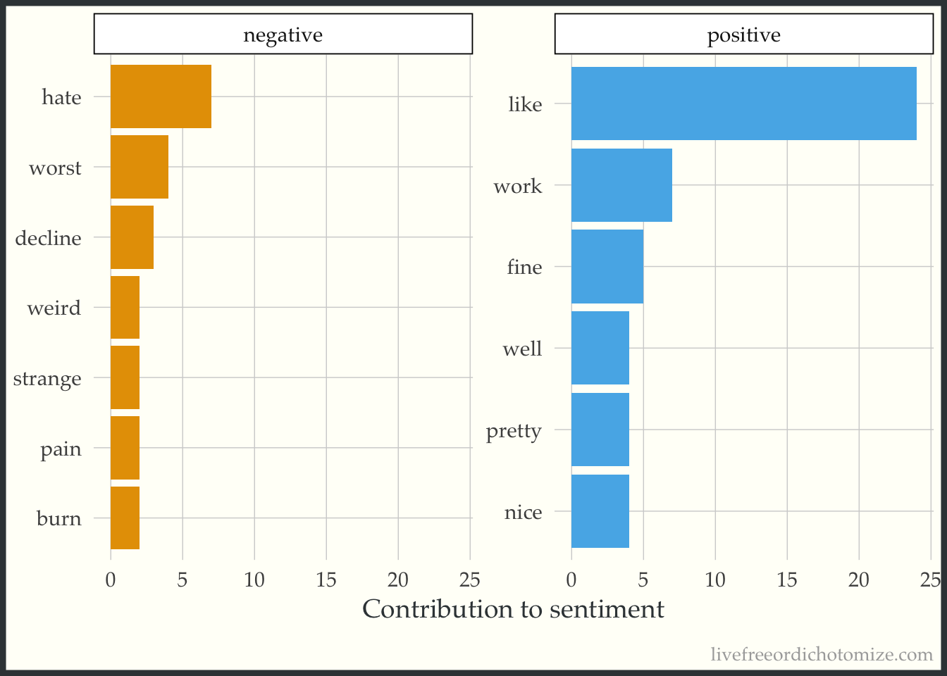
Coming at you 🔥 from the fresh-off-the-press Text Mining with R, let’s do a little sentiment analysis to see how folks were feeling while replying to this curiosity.
Check out an example just like this and more examples on the Text Mining with R website
library("tidytext")
#this will drop links & symbols
drop_pattern <- "https://t.co/[A-Za-z\\d]+|http://[A-Za-z\\d]+|&|<|>|RT|https|ht"
unnest_pattern <- "([^A-Za-z_\\d#@']|'(?![A-Za-z_\\d#@]))"
all_replies %>%
mutate(text = stringr::str_replace_all(text, drop_pattern, "")) %>%
unnest_tokens(word,
text,
token = "regex",
pattern = unnest_pattern) %>%
inner_join(get_sentiments("bing"), by = "word") %>%
count(word, sentiment, sort = TRUE) %>%
ungroup() %>%
group_by(sentiment) %>%
top_n(5) %>%
ungroup() %>%
mutate(word = reorder(word, n)) %>%
ggplot(aes(word, n, fill = sentiment)) +
geom_col(show.legend = FALSE) +
facet_wrap(~sentiment, scales = "free_y") +
labs(y = "Contribution to sentiment",
x = NULL) +
coord_flip()
It looks like the poll represents the people! There seems to generally be more positive sentiment, with some strongly worded negative sentiment snuck in there 😉.