The traveling metallurgist
TLDR: I made a thing that moves and has sliders and stuff. It’s down here.
Currently I am taking a class titled “Advanced Statistical Computing” taught here at Vanderbilt by Chris Fonnesbeck. The class is a fantastic whirlwind tour so far of some common optimization algorithms used in statistical computing. One of the algorithms I have found particularly fascinating is the “simulated annealing” algorithm. The whole algorithm is explained much better than I can do in the freely available Jupyter notebook for the lecture. The inspiration for simulated annealing is from, unsurprisingly, annealing. Which is the act of heating up a metal and then slowly cooling it down to allow the atoms inside to find their optimal arrangement for strength before being locked into place. 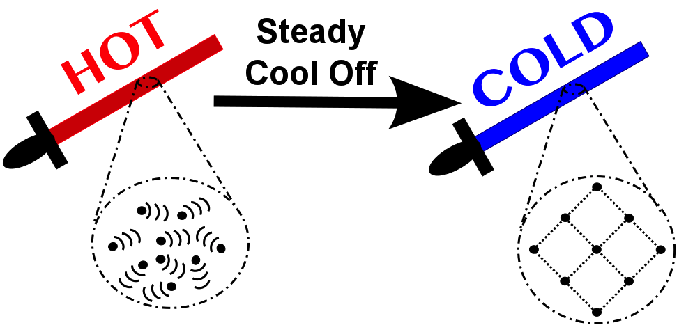 Why annealing is valuable in metullurgy. Source.
Simulated annealing attempts to replicate this process but for optimizing some loss function. A loss function in this context is any measurable outcome/performance of a model. For instance this could be the performance of a model via AIC, or the log-likelihood, or it could be the number of mistakes a robot makes in navigating a maze. The types of problems simulated-annealing is typically used for are those who have so many possible solutions that brute force figuring out the solution would be essentially impossible.
How the algorithm works in a very broad sense is that a starting state is chosen (often at random) and the performance is measured via your loss function of choice. After this, the solution (such as parameters included in your model) is mutated randomly and the performance of the new mutated model is calculated. If it is better than your previous solution, you “accept” the new solution. We could stop right here and have a good method for optimization, the problem is that this will have a tendency to get stuck in a local minimum or a solution that is better than any solution ‘close by’ or within range of a single mutation, but not necessarily the best overall solution.  Source What simulated annealing does to combat this is it will sometimes accept new permutations of the solution that perform worse than the previous. By doing this it explores the solution space and has the potential to work its way out of those pesky local minimum. Again though, there is a problem, if we always are willing to accept worse solution, how will we ever narrow down and find the best solution once we do get nearby the true global minimum? This is where the inspiration really takes hold. What the algorithm does is it slowly, as the generations of model permutation progress, gets more and more conservative with the solutions it accepts. For instance, at the beginning almost any solution will be accepted, causing the algorithm to explore a large portion of the solution space, but then it slowly dials back this willingness to bounce around with the hopes that it has bounced into the vicinity of the true global minimum. The way that this willingness to bounce is controlled is called the ‘temperature.’
Setting an Itinerary
One of the classic problems that is infeasible to compute exactly is the traveling salesman problem. A salesman has a list of cities he needs to visit to do salesman things in, but he wants to minimize the amount of time he spends traveling between all the cities so he sets out trying to figure out the optimal route that will minimize his traveling distance. Two cities is easy, there’s just one path so no choice, adding another city is also fine, there’s only two ways to do this, 1,2,3,1, or 1,3,2,1 (he lives in city 1 so he always starts and returns there.) Even four cities isn’t bad, you just throw the fourth city into one of three slots in the previous paths ({1,-,-,4,1}, {1,-,4,-,1}, {1,4,-,-,1}) for a total of 6 possible routes. Five cities starts to get a little bit trickier, you have to add the fifth city into one of 4 possible slots in the six previous routes, this continues such that if you have \(n\) cities and add an \((n + 1)^{th}\) city, the possible number of routes you have to consider is \(n!\), which is a large number past 5. \(25! = 1.55 * 10^{25}\) Even though our computers are super duper fast, they can’t do that many calculations in the human (or universe’s) lifespan.
Simulated annealing is a way of solving this problem. The best ways tend to approach it as a graph problem, but this works too Essentially what you can do is start with a random route that passes through every city, then randomly choose a given city in the route path and move it. So say your route was 1,2,3, 4 ,5, you could take city 4 and randomly place it somewhere else to get a new route such as 1, 4, 2, 3, 5. The loss function in this case is total distance traveled.
This is all fun and easy to write/read about, but I find these algorithms make more sense when I can get in and watch them work and fiddle with them, which is why I have made an interactive that allows you to watch simulated annealing try and solve the traveling salesman problem.
Click to add or remove cities. Use slider to take manual control of the temperature schedule. To slow down the visualization increase the step delay.
If you prefer you can just let it run and it should (but not always) do a good job of finding a sensible route through the randomly generated cities, but I encourage you to poke and prod it and ask questions. Here are just a few that I’ve asked myself while building it:
- Can you fool the algorithm by adding (click or tap anywhere without a city) or deleting cities (click or tap on an existing city)?
- Try deleting cities until you have a perimeter, or an easy to solve problem, and then see if you can fool the algorithm by putting a city smack in the middle.
- Can you come up with a cooling routine that allows the algorithm to converge faster than the default (exponential) one?
- The cooling function will auto-run to cool down exponentially, but you can take control of it.
- What happens if you pulse the temperature?
- What is the relationship between a decrease in the cooling rate and the model performance?
- Should the model try and flip two cities each generation or one, or five?
- Why would increasing the number of flips each generation not necessarily make the model converge faster?
- When might it be a good decision?