MCMC and the case of the spilled seeds
Earlier this month I did a post on simulated annealing, an algorithm that I learned in the class I’m currently taking: Advanced Statistical Computing taught by Chris Fonnesbeck here at Vanderbilt. Recently we have moved on to more traditionally “statistics” algorithms, and one that Dr. Fonnesbeck is particularly well versed in, Markov-Chain Monte-Carlo (or MCMC). Dr. Fonnesbeck is the creator of the very popular python library pymc. In this post I hope to elucidate what MCMC is, why we need it, and show how one particular way of doing it (the metropolis hastings sampler) works.
What is MCMC?
If you want to sound smart, next time someone asks you what you like thinking about, say “Markov-Chain Monte-Carlo”,  I always think of Marco Polo when I think of Monte-Carlo. it’s a nice long mouthful of sciency soundings words that cause most people to zone out after about two syllables. What does it mean in normal language? Markov-Chain
  Markov Chains are used in lots of cool places. For instance, generating fake text.refers to the idea of a sequence of draws such that the only thing that all you need to know about what the next value will be is the one just prior to it. Think of it like the mathematical equivalent to Dory from Finding Nemo, once she’s in a place she has no memory of where she was before and her next action is based only upon her current situation. Monte-Carlo refers to the act of estimating something by simulation. Basically the concept of, if you want to understand a process, repeat it a bunch of times and look at the aggregate behavior. Another example of monte carlo methods in statistics can be seen in my previous post Wait, what are P-values?
Why do we need MCMC?
When I say ‘we’ in this context I mean Bayesian statisticians (which, while reading this article, you are), or statisticians that like to think in terms of probabilities instead of frequencies. I won’t go into the Bayesian vs Frequentest debate here as it would be way too long and boring, but there’s plenty of literature on it to be found. Like all of life’s problems, stack overflow has a good answer.
A huge reason why Bayesian statistics was so unpopular up until very recently is because when calculating the “posterior” distribution a large portion of the time the math simply wasn’t tractable. To see what I mean it helps to think about the form of a posterior distribution.
\[\begin{aligned} \text{Posterior of parameter} &= \frac{P(\text{data given parameter}) \cdot P(\text{parameter})}{\int P(\text{data given parameter}) \cdot P(\text{parameter})} \end{aligned}\]
The top of this equation is rather straightforward, you simply multiply the distribution you believe your data is derived from by the distribution you believe the true parameter of interest follows. E.g. the density function of the normal distribution multiplied by the density function of another normal representing the distribution of the mean of the data’s distribution. The problem comes with the integral below. Since it’s integrating over the entire possible space of the parameter of interest it is simply a constant, but finding what constant it is is tricky. Even if you did some optimization method to find it, you still have the problem that most of the math you would want to do with the posterior distribution involves taking an integral over the same values again so just having the normalizing constant is not of much help. One of my mottos in life is, ‘if the math is at all hard, just simulate it’, which turns out to be rather helpful in a lot of statistics.
What MCMC does to solve this is, using the numerator of that posterior (also known as the un-normalized posterior), it generates data that fits the distribution, once you have a bunch of samples of data from a given distribution you can do almost any inference you would desire. Want to know how often you would see parameter values greater than \(p\)? Just take the samples MCMC generated for you and count how many were above \(p\) and divide by the total number of samples.
How does MCMC work?
There are a few ways of performing MCMC and the way I am going to demonstrate here (Metropolis-Hastings) is not the state of the art,For a fantastic overview of the more cutting edge Hamiltonian Monte-Carlo methods, I recomend taking a look at the lecture notes for my class on github. however, it is the most straightforward and intuitive method of MCMC and I think is valuable to understand. Essentially the algorithm works like this (I am going to demonstrate for a single parameter but the concept extends to multiple dimensions with the exact same logic):
- Choose a random initial value of the parameter of interest \(\theta_0\)
- Calculate the value of your un-normalized posterior multiplied by this \(\theta_0\) and remember it (\(P_0\)).
- Randomly jump from \(\theta_0\) to some new value nearby, \(\theta_1\).
- Calculate the value of your un-normalized posterior at this new location, \(P_1\).
- Choose to move to \(\theta_1\) with probability proportional to how much better or worse \(P_1\) is than \(P_0\), if you don’t move make your next \(\theta\) a duplicate of \(\theta_0\).
- Repeat steps 3-5 for a while, recording each step’s \(\theta_i\).
- Treat all of your recorded \(\theta\)s as observations from the posterior distribution and relish in the wonderful bayesianness of this whole endeavor.
Like all good algorithms there are knobs to turn. For instance, how big of a jump your algorithm takes at any given step is very important. Too large and it will almost never be accepted and the algorithm will take forever to converge to the posterior, too small and the steps nearby each other will be too correlated and the algorithm will focus too much on a given area of the posterior. For metropolis hastings the sweet spot seems to be making your jumps distributed widely enough to have roughly 23% of the proposals accepted. Optimal Acceptance Rates for Metropolis Algorithms:Moving Beyond 0.234 is a good paper to read if you’re interested in how these things are calculated and why that single number is still not perfect.
However, I’ve just spewed a bunch of words and complex math terms at you, and I had the same thing done to me many times before I truly understood the algorithm. What got me to understand it? Playing with the knobs and seeing how it works. I’ve tried to distill the algorithm to its fundamental parts below for you to tinker with yourself.
Problem Setup
Let’s say you have a bird feeder on your porch and you have two bird species that visit it: a Cardinal 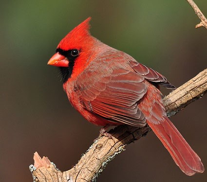 Cardinal and a Carolina Wren
 Carolina Wren. You have noticed that there tend to be a lot of seeds spilled on the ground around the feeder. This annoys you because you spent a lot of money on those seeds and those ungrateful birds are wasting a lot of them. You decide to Google the problem and find a handy website that lays out the seed spilling habits of both the Cardinal and the Carolina Wren. This site says that the Cardinal’s seed spillage amount per feeding follows a normal distribution with a mean of 65 and a standard deviation of 10, and the Carolina Wren’s happen to follow a normal distribution with a mean of 85 seeds and a standard deviation of 10 as well. Sometimes the birds carry seeds with them and thus can possibly spill negative seeds, so this truly is normal…
The thing is, you want to know what the makeup of your bird spillers are so you can know which bird species to be more mad at. You put a scale beneath the feeder that can automatically measure the spillage from a single feeding. It’s a single bird feeder so only one bird feeds at a time. So you have data on how much seed was spilled at each feeding, and you know the distribution of spillage for each bird species, but you have a job so you can’t actually sit there and watch the birds feed, plus you understand that the real distribution of birds feeding probably is just that, a distribution. What can you do? You can do Bayesian statistics!
The data likelihood is a normal mixture: \(L(\delta|\text{seeds}) = \delta N(\text{Cardinal}) + (1 - \delta)N(\text{Carolina Wren})\)
You don’t have any real idea about which bird will be more likely so your prior is a uniform distribution over the range 0 and 1 (\(U(0,1)\)).
Turns out they actually make products to catch spilled seeds so this convoluted example isn’t too crazy. 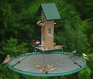
Your proposal distribution is another random uniform with a width of 2, aka \(U(-1,1)\).
You can fiddle with the sliders below to change the true mean of seeds dropped by two birds, the true percentage of times the Cardinal is at the feeder, the size of your observation data and how wide your proposals are. Play around with the dials to see how the algorithm reacts. The plot below will show the real-time results of MCMC running including the current 95% credible interval (aka what people think a confidence interval is) and the acceptance rate. The algorithms proposed values for the proportion that are rejected are displayed as red circles.
Here are a few experiments you may want to run to explore the algorithm’s behavior:
- Can you fool the credible interval? Try setting the true means of the two birds very close and your number of observations really low, intuitively this will be much harder to discern between each bird in the data.
- See how increasing the number of observations results in a skinnier posterior.
- If you’re really adventurous, try forking the code for this simulation from github and switching the prior to a beta distribution in this file. The beta will allow you to give opinionated priors about the distribution of the parameter of interest, but sometimes at a cost of accuracy.
Still confused? MCMC is non-trivial to say the least, so don’t feel bad if you don’t get it. Please let me know in the comments or on twitter what is confusing so I can try and make this explanation better!