Survival Model Detective: Part 1

A paper by Grein et al. was recently published in the New England Journal of Medicine examining a cohort of patients with COVID-19 who were treated with compassionate-use remdesivir. This paper had a very cool figure - here’s how to recreate it in R!

A paper by Grein et al. was recently published in the New England Journal of Medicine examining a cohort of patients with COVID-19 who were treated with compassionate-use remdesivir. There are two things that were interesting about this paper:

1. They had a very neat figure that included tons of information about their cohort
2. The primary statistical analysis was not appropriately done

This post focuses on the very neat figure!

Figure 2

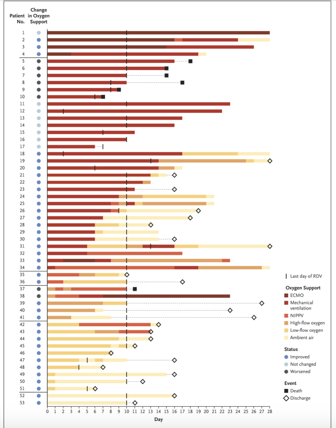
Figure 2 in the original paper shows the changes in oxygen-support status from baseline for each of the 53 patients. This figure includes information about:

• The duration of follow up for each individual patient
• Each patient’s oxygen trajectory
• Each patient’s ultimate outcome (death, discharged, censored)

You can construct a whole dataset from this (and I did!) - you can find it on my GitHub.

Below is code to recreate their Figure 2 using #rstats 😎.

library(tidyverse)
d <- read_csv("https://raw.githubusercontent.com/LucyMcGowan/nejm-grein-reanalysis/master/data/data-fig-2.csv")

long_dat <- d %>%
  pivot_longer(day_1:day_36)

cats <- tibble(
  value = 1:6,
  cat = factor(c("Ambient air", "Low-flow oxygen", "High-flow oxygen", "NIPPV", 
                 "Mechanical ventilation", "ECMO"),
               levels = c("ECMO", "Mechanical ventilation", "NIPPV", 
                          "High-flow oxygen", "Low-flow oxygen", "Ambient air"))
)
long_dat %>%
  left_join(cats, by = "value") %>%
  filter(!is.na(value)) %>%
  mutate(day_oxy = as.numeric(gsub("day_", "", name)) - 1,
         day_oxy = ifelse(day_oxy > 28, 28, day_oxy),
         day = ifelse(day > 28, 28, day),
         patient = factor(patient, levels = 53:1),
         event = ifelse(event == "censor", NA, event)
  ) %>%
  ggplot(aes(x = patient, y = day_oxy, fill = cat)) +
  geom_segment(aes(x = patient, xend = patient,
                   y = 0, yend = day - 0.5), lty = 3) +
  geom_tile(width = 0.5) + 
  scale_fill_manual("Oxygen support",
                    values = c("#7D3A2C", "#AA3B2F", "#D36446", "#DEA568", 
                               "#F5D280", "#FCEEBC")) +
  geom_point(aes(x = patient, y = day - 0.5, shape = event)) +
  scale_shape_manual("Event", values = c(15, 5),
                     labels = c("Death", "Discharge", "")) +
  guides(fill = guide_legend(override.aes = list(shape = NA), order = 1)) +
  coord_flip() +
  labs(y = "day", x = "") +
  theme_classic()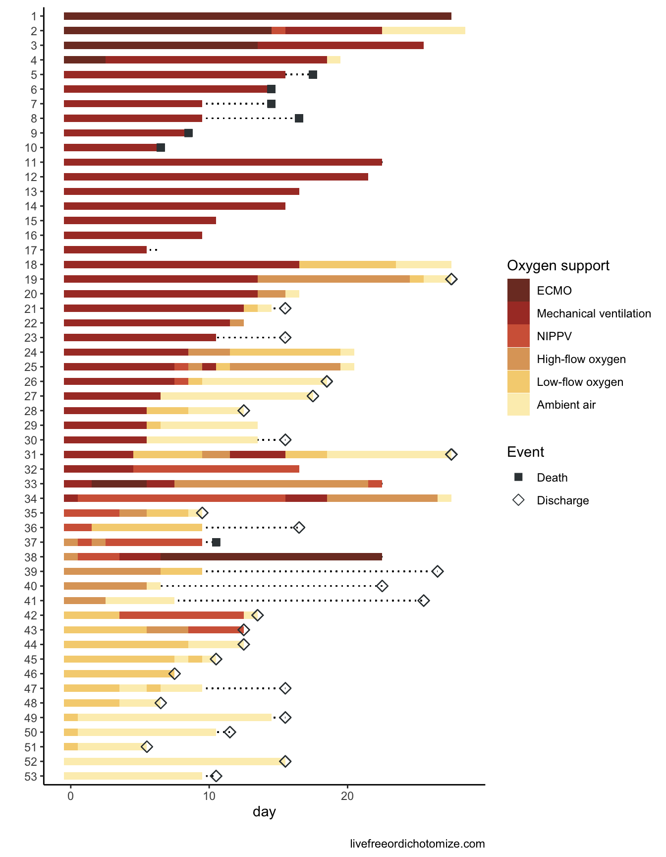

I definitely applaud the authors for making this so accessible! Check out Part 2 to see a bit about how their statistics could be improved.