library(tidyverse)
library(broom)
library(mice)

n <- 1000

set.seed(928)

data <- tibble(
  c_x = rnorm(n, sd = 0.71),
  x = c_x + rnorm(n, sd = 0.71),
  c_y = rnorm(n),
  y = x + c_y + rnorm(n),
  noise = rnorm(n),
  x_miss = rbinom(n, 1, 1 / (1 + exp(-(c_x + c_y)))),
  x_obs = ifelse(
    x_miss,
    NA,
    x
  )
)Are two wrong models better than one? Missing data style
rstats
simulations
missing data
Would imputing + fitting an outcome model using the wrong variables be better than just fitting the wrong outcome model? Let’s investigate!
After my previous post about missing data, Kathy asked on Twitter whether two wrong models (the imputation model + the outcome model) would be better than one (the outcome model alone).
Without doing any of the math, I’d guess the assumption of correctly spec the model also has a bigger impact in the CC analysis.
You need correct spec in MI, twice, but trade off that potential bias for higher prec.
This is a great question! I am going to investigate via a small simulation (so the answer could be “it depends”, but at least we will know how it seems to work in this very simple case) 😆.
Ok so here I have some predictor, x that is missing 50% of the time, dependent on c_x and c_y. The right imputation model would have c_x, the right outcome model needs c_y. Unfortunately, we only have access to one, which we will try to use in our imputation model (and outcome model). Let’s see whether two (wrong) models are better than one!
A “correct” model will be one that estimates that the coefficient for x is 1.
We only have c_x
Ok first let’s look at the whole dataset.
mod_full_c_x <- lm(y ~ x + c_x, data = data) |>
  tidy(conf.int = TRUE) |>
  filter(term == "x") |>
  select(estimate, conf.low, conf.high)

mod_full_c_x
# A tibble: 1 × 3
estimate conf.low conf.high
<dbl> <dbl> <dbl>
1 1.01 0.877 1.14This checks out! c_x basically does nothing for us here, but because c_y is not actually a confounder (it just informs the missingness & y, which we aren’t observing here), we are just fine estimating our “wrong” model in the fully observed data. Now let’s do the “complete cases” analysis.
data_cc <- na.omit(data)
mod_cc_c_x <- lm(y ~ x + c_x, data = data_cc) |>
  tidy(conf.int = TRUE) |>
  filter(term == "x") |>
  select(estimate, conf.low, conf.high)

mod_cc_c_x
# A tibble: 1 × 3
estimate conf.low conf.high
<dbl> <dbl> <dbl>
1 0.999 0.812 1.19This does fine! Now let’s do some imputation. I am going to use the mice package.
imp_data_c_x <- mice(
  data,
  m = 5,
  method = "norm.predict",
  formulas = list(x_obs ~ c_x),
  print = FALSE)
Ok let’s compare how this model does “alone”.
mod_imp_c_x <- with(imp_data_c_x, lm(y ~ x_obs)) |>
  pool() |>
  tidy(conf.int = TRUE) |>
  filter(term == "x_obs") |>
  select(estimate, conf.low, conf.high)

mod_imp_c_x
estimate conf.low conf.high
1 1.026666 0.9042858 1.149046Great! This was the right model, so we would expect this to perform well.
Now what happens if we adjust for c_x in addition in the outcome model:
mod_double_c_x <- with(imp_data_c_x, lm(y ~ x_obs + c_x)) |>
  pool() |>
  tidy(conf.int = TRUE) |>
  filter(term == "x_obs") |>
  select(estimate, conf.low, conf.high)

mod_double_c_x
estimate conf.low conf.high
1 0.9991868 0.7968509 1.201523The right imputation model with the wrong outcome model is fine!
We only have c_y
Ok first let’s look at the whole dataset.
mod_full_c_y <- lm(y ~ x + c_y, data = data) |>
  tidy(conf.int = TRUE) |>
  filter(term == "x") |>
  select(estimate, conf.low, conf.high)

mod_full_c_y
# A tibble: 1 × 3
estimate conf.low conf.high
<dbl> <dbl> <dbl>
1 1.01 0.946 1.08Looks good! Now let’s do the “complete cases” analysis.
mod_cc_c_y <- lm(y ~ x + c_y, data = data_cc) |>
  tidy(conf.int = TRUE) |>
  filter(term == "x") |>
  select(estimate, conf.low, conf.high)

mod_cc_c_y
# A tibble: 1 × 3
estimate conf.low conf.high
<dbl> <dbl> <dbl>
1 1.01 0.909 1.11Great! It works. This shows that as long as we have the right outcome model we can do complete case analysis even if the data is missing not at random (cool!). Now let’s do some imputation.
imp_data_c_y <- mice(
  data,
  m = 5,
  method = "norm.predict",
  formulas = list(x_obs ~ c_y),
  print = FALSE)
Ok let’s compare how this model does “alone”.
mod_imp_c_y <- with(imp_data_c_y,lm(y ~ x_obs)) |>
  pool() |>
  tidy(conf.int = TRUE) |>
  filter(term == "x_obs") |>
  select(estimate, conf.low, conf.high)

mod_imp_c_y
estimate conf.low conf.high
1 0.6888255 0.527796 0.849855Oh no, very bad! The wrong imputation model is worse than complete case! By a lot! This estimate is off by 0.31. Does conditioning on c_y help us at all?
mod_double_c_y <-  with(imp_data_c_y, lm(y ~ x_obs + c_y)) |>
  pool() |>
  tidy(conf.int = TRUE) |>
  filter(term == "x_obs") |>
  select(estimate, conf.low, conf.high)

mod_double_c_y
estimate conf.low conf.high
1 1.009655 0.8887281 1.130582Phew, the wrong imputation model with the wrong outcome model is back to being fine.
What if both are wrong?
Ok, what if we just had our useless variable, noise.
mod_full_noise <- lm(y ~ x + noise, data = data) |>
  tidy(conf.int = TRUE) |>
  filter(term == "x") |>
  select(estimate, conf.low, conf.high)

mod_full_noise
# A tibble: 1 × 3
estimate conf.low conf.high
<dbl> <dbl> <dbl>
1 0.992 0.898 1.09This is fine! c_x and c_y aren’t confoudners so we can estimate the coefficent for x without them – noise doesn’t do anything, but it also doesn’t hurt. What about complete case?
mod_cc_noise <- lm(y ~ x + noise, data = data_cc) |>
  tidy(conf.int = TRUE) |>
  filter(term == "x") |>
  select(estimate, conf.low, conf.high)

mod_cc_noise
# A tibble: 1 × 3
estimate conf.low conf.high
<dbl> <dbl> <dbl>
1 0.887 0.748 1.03Oops! We’ve got bias (as expected!) – we end up with a biased estimate by ~0.11.
What if we build the (wrong) imputation model?
imp_data_noise <- mice(
  data,
  m = 5,
  method = "norm.predict",
  formulas = list(x_obs ~ noise),
  print = FALSE)
Ok let’s compare how this model does “alone”.
mod_imp_noise <-  with(imp_data_noise, lm(y ~ x_obs)) |>
  pool() |>
  tidy(conf.int = TRUE) |>
  filter(term == "x_obs") |>
  select(estimate, conf.low, conf.high)

mod_imp_noise
estimate conf.low conf.high
1 0.8807755 0.7217368 1.039814This is also wrong (womp womp!) What if we try two wrong models?
mod_double_noise <-  with(imp_data_noise,lm(y ~ x_obs + noise)) |>
  pool() |>
  tidy(conf.int = TRUE) |>
  filter(term == "x_obs") |>
  select(estimate, conf.low, conf.high)

mod_double_noise
estimate conf.low conf.high
1 0.8865363 0.7275635 1.045509Nope 😢. Two wrong models here are not better than one! It’s worse! Womp womp.
Let’s put these all together:
bind_rows(
  mod_full_c_x,
  mod_full_c_y,
  mod_full_noise,
  mod_cc_c_x,
  mod_cc_c_y,
  mod_cc_noise,
  mod_imp_c_x,
  mod_imp_c_y,
  mod_imp_noise,
  mod_double_c_x,
  mod_double_c_y,
  mod_double_noise
) |>
  mutate(
    mod = factor(c("Full data with c_x",
                   "Full data with c_y",
                   "Full data with noise",
                   "Complete case with c_x",
                   "Complete case wtih c_y",
                   "Complete case with noise",
                   "Imputation with c_x",
                   "Imputation with c_y",
                   "Imputation with noise",
                   "Two models with c_x",
                   "Two models with c_y",
                   "Two models with noise" ),
                 levels = c("Full data with c_x",
                            "Complete case with c_x",
                            "Imputation with c_x",
                            "Two models with c_x",
                            "Full data with c_y",
                            "Complete case wtih c_y",
                            "Imputation with c_y",
                            "Two models with c_y",
                            "Full data with noise",
                            "Complete case with noise",
                            "Imputation with noise",
                            "Two models with noise" )),
    mod = fct_rev(mod),
  ) -> to_plot

ggplot(to_plot, aes(x = estimate, xmin = conf.low, xmax = conf.high, y = mod)) +
  geom_pointrange() +
  geom_vline(xintercept = 1, lty = 2)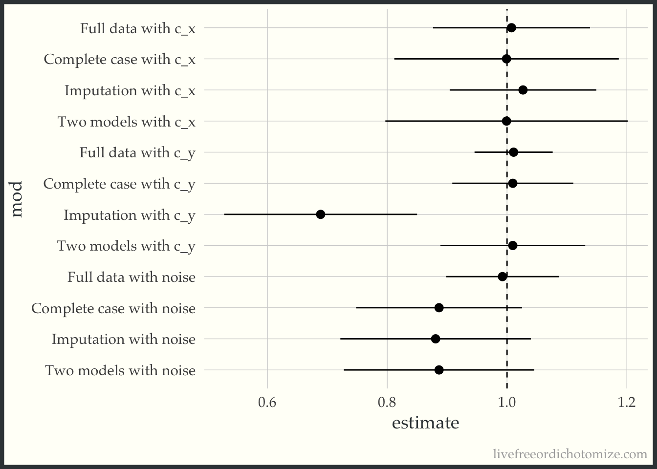
So there you have it, two wrong models are rarely better than one.
Addendum!
In writing this post, I found that I was getting biased results when I was correctly specifying my imputation model when using the {mice} defaults (which is why the code above specifies norm.predict for the method, forcing it to use linear regression, as the data were generated). I didn’t understand why this is happening until some helpful friends on Twitter explained it (thank you Rebecca, Julian, and Mario. I’ll show you what is happening and then I’ll show a quick explanation. Let’s try to redo the imputation models using the defaults:
imp_default_c_x <- mice(
  data,
  m = 5,
  formulas = list(x_obs ~ c_x),
  print = FALSE)
mod_imp_c_x <- with(imp_default_c_x, lm(y ~ x_obs)) |>
pool() |>
tidy(conf.int = TRUE) |>
filter(term == "x_obs") |>
select(estimate, conf.low, conf.high)
mod_imp_c_x estimate conf.low conf.high
1 0.7353276 0.6194273 0.8512279Bad!
mod_double_c_x <-  with(imp_default_c_x, lm(y ~ x_obs + c_x)) |>
  pool() |>
  tidy(conf.int = TRUE) |>
  filter(term == "x_obs") |>
  select(estimate, conf.low, conf.high)

mod_double_c_x
estimate conf.low conf.high
1 0.4602637 0.30023 0.6202974Even worse!!
imp_default_c_y <- mice(
  data,
  m = 5,
  formulas = list(x_obs ~ c_y),
  print = FALSE)
mod_imp_c_y <- with(imp_default_c_y, lm(y ~ x_obs)) |>
pool() |>
tidy(conf.int = TRUE) |>
filter(term == "x_obs") |>
select(estimate, conf.low, conf.high)
mod_imp_c_y estimate conf.low conf.high
1 0.3405789 0.1126282 0.5685295YIKES!
mod_double_c_y <-  with(imp_default_c_y, lm(y ~ x_obs + c_y)) |>
  pool() |>
  tidy(conf.int = TRUE) |>
  filter(term == "x_obs") |>
  select(estimate, conf.low, conf.high)

mod_double_c_y
estimate conf.low conf.high
1 0.5128878 0.3216547 0.7041208Better since we are conditioning on c_y (but still bad!)
imp_default_noise <- mice(
  data,
  m = 5,
  formulas = list(x_obs ~ noise),
  print = FALSE)
mod_imp_noise <- with(imp_default_noise, lm(y ~ x_obs)) |>
pool() |>
tidy(conf.int = TRUE) |>
filter(term == "x_obs") |>
select(estimate, conf.low, conf.high)
mod_imp_noise estimate conf.low conf.high
1 0.4076967 0.2352155 0.5801779EEK!
mod_double_noise <-  with(imp_default_noise,lm(y ~ x_obs + noise)) |>
  pool() |>
  tidy(conf.int = TRUE) |>
  filter(term == "x_obs") |>
  select(estimate, conf.low, conf.high)

mod_double_noise
estimate conf.low conf.high
1 0.4124791 0.2497624 0.5751959Just as bad..
Let’s put those in the original plot:
bind_rows(
  mod_full_c_x,
  mod_full_c_y,
  mod_full_noise,
  mod_cc_c_x,
  mod_cc_c_y,
  mod_cc_noise,
  mod_imp_c_x,
  mod_imp_c_y,
  mod_imp_noise,
  mod_double_c_x,
  mod_double_c_y,
  mod_double_noise
) |>
  mutate(
    mod = factor(c("Full data with c_x",
                   "Full data with c_y",
                   "Full data with noise",
                   "Complete case with c_x",
                   "Complete case wtih c_y",
                   "Complete case with noise",
                   "Default Imputation with c_x",
                   "Default Imputation with c_y",
                   "Default Imputation with noise",
                   "Two models with c_x",
                   "Two models with c_y",
                   "Two models with noise" ),
                 levels = c("Full data with c_x",
                            "Complete case with c_x",
                            "Default Imputation with c_x",
                            "Two models with c_x",
                            "Full data with c_y",
                            "Complete case wtih c_y",
                            "Default Imputation with c_y",
                            "Two models with c_y",
                            "Full data with noise",
                            "Complete case with noise",
                            "Default Imputation with noise",
                            "Two models with noise" )),
    mod = fct_rev(mod),
  ) -> to_plot

ggplot(to_plot, aes(x = estimate, xmin = conf.low, xmax = conf.high, y = mod)) +
  geom_pointrange() +
  geom_vline(xintercept = 1, lty = 2)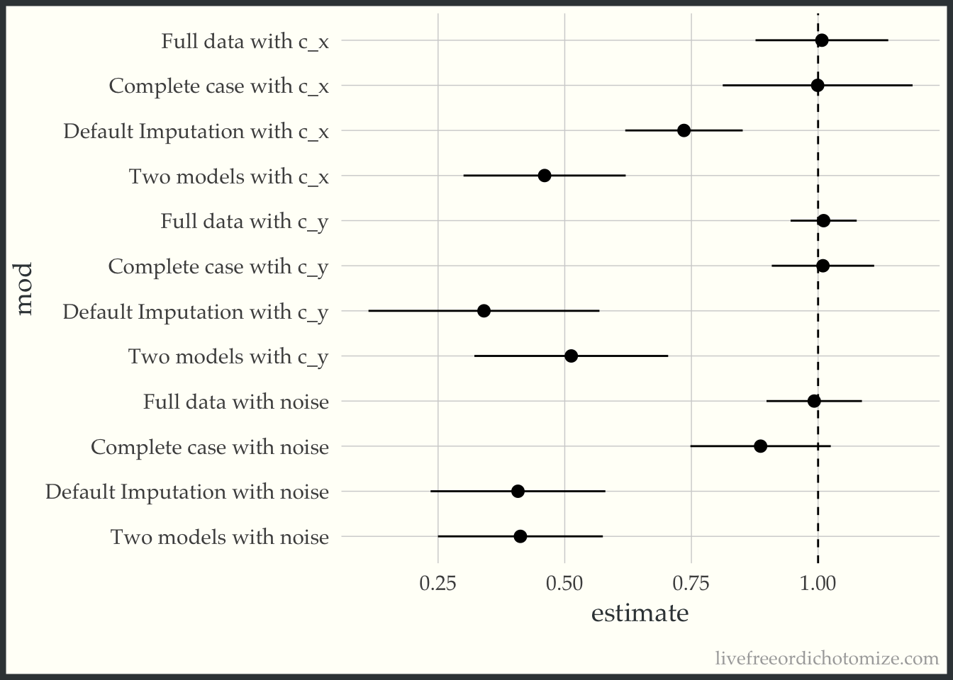
AHH! This makes me so scared of imputation!!
Rebecca Andridge’s tweet finally helped me see why this is happening. The way the missing data is generated, larger values of c_x have a higher probability of missingness, and for particularly high values of c_x that probability is almost 1.
ggplot(data, aes(x = x, y = y, color = factor(x_miss))) +
  geom_point() +
  geom_vline(xintercept = 2.31, lty = 2) +
  labs(color = "missing")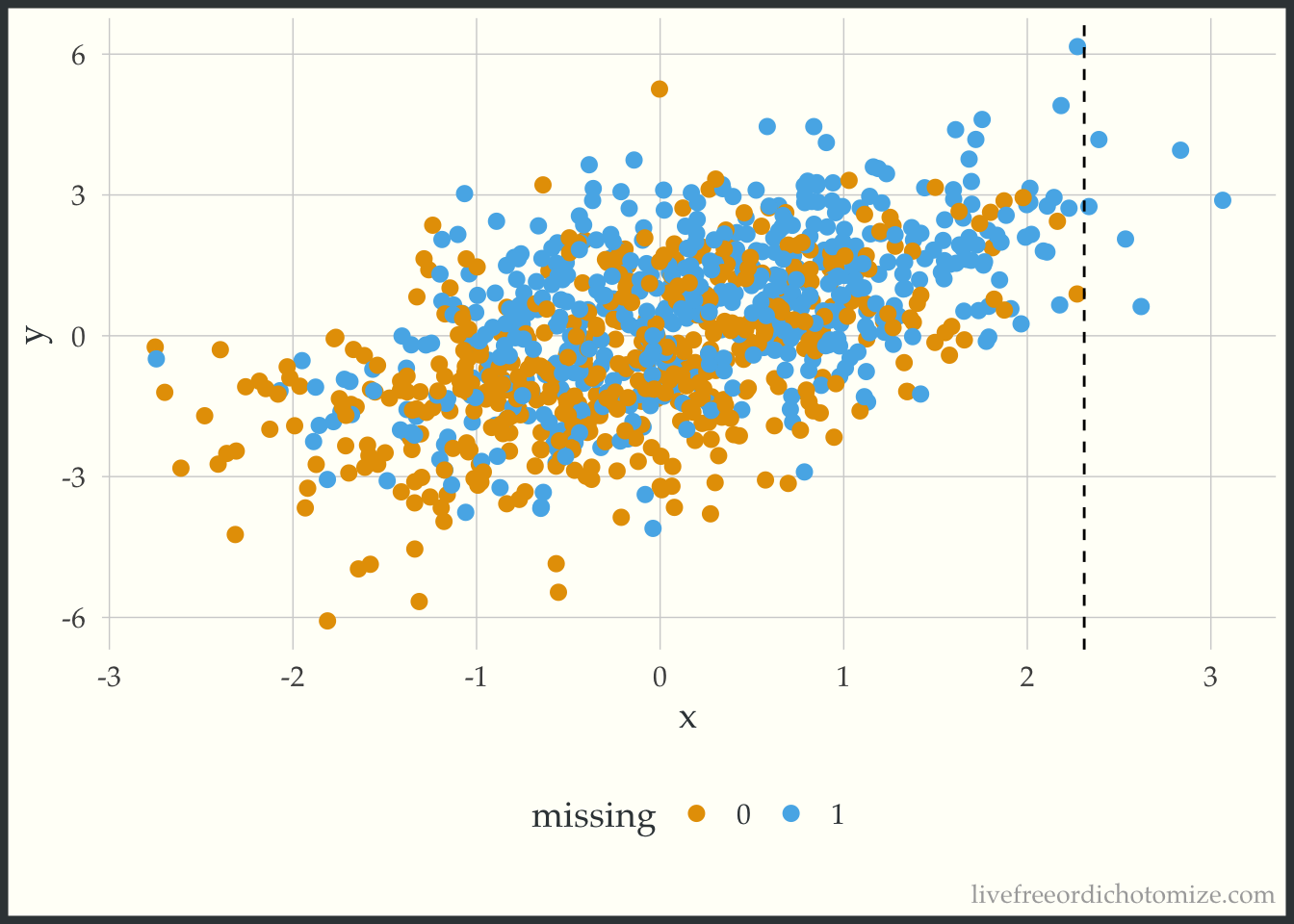
Take a look at the plot above. We have no non-missing x values that are greater than 2.3. The way predictive mean matching (the default {mice} method) works is it finds the observation(s) that have the closest predicted value to the observation that is missing a data point and gives you that non-missing data point’s value. So here, we are essentially truncating our distribution at 2.3, since that is the highest value observed. Any value that would have been higher is going to be necessarily too small instead of the right value (this is different from the linear model method used in the first part of this post, which allows you to extrapolate). This is supposed to be a less biased approach, since it doesn’t allow you to extrapolate beyond the bounds of your observed data, but it can actually induce bias when you have pockets of missingness with no observed xs (which I would argue might happen frequently!). Here is an example of one of the imputed datasets, notice nothing is above that 2.3 line!
ggplot(complete(imp_default_c_x), aes(x = x_obs, y = y, color = factor(x_miss))) +
  geom_point() +
  scale_x_continuous(limits = c(-2.8, 3.1)) +
  geom_vline(xintercept = 2.31, lty = 2) +
labs(color = "imputed") 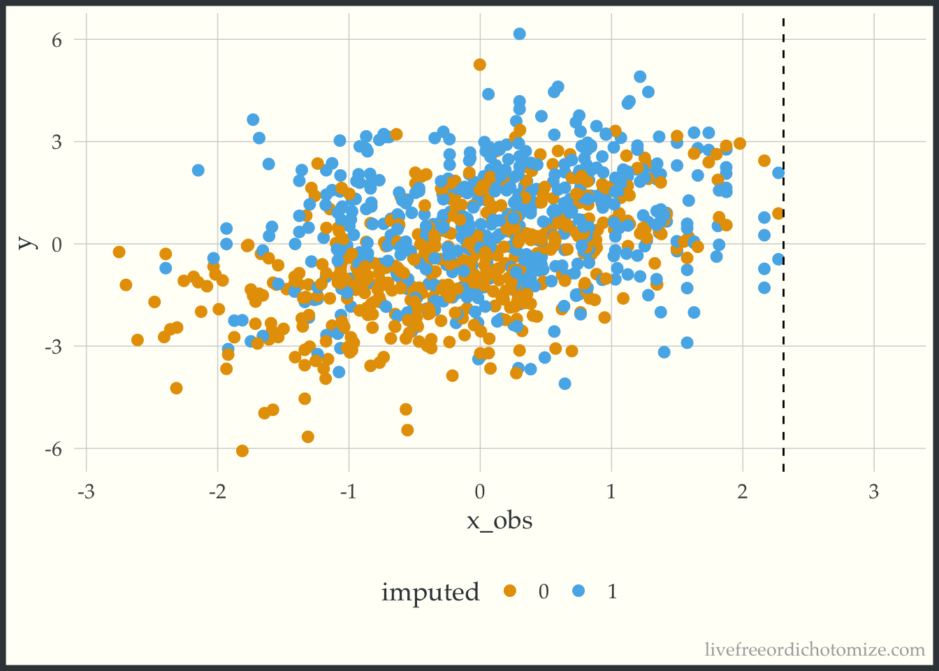
What if we use y in the imputation models
Including y in the imputation model is definitely recommended, as was hammered home for me by the wonderful Frank Harrell, but I’m not sure this recommendation has permeated through the field yet (although this paper re-iterating this result just came out yesterday so maybe it is!).
Let’s see how that improves our imputation models:
imp_y_c_x <- mice(
  data,
  m = 5,
  formulas = list(x_obs ~ c_x + y),
  print = FALSE)
mod_imp_c_x <- with(imp_y_c_x, lm(y ~ x_obs)) |>
pool() |>
tidy(conf.int = TRUE) |>
filter(term == "x_obs") |>
select(estimate, conf.low, conf.high)
mod_imp_c_x estimate conf.low conf.high
1 1.034138 0.9109341 1.157343Beautiful!
mod_double_c_x <-  with(imp_y_c_x, lm(y ~ x_obs + c_x)) |>
  pool() |>
  tidy(conf.int = TRUE) |>
  filter(term == "x_obs") |>
  select(estimate, conf.low, conf.high)

mod_double_c_x
estimate conf.low conf.high
1 1.08074 0.8772936 1.284186A bit worse, but not bad!
imp_y_c_y <- mice(
  data,
  m = 5,
  formulas = list(x_obs ~ c_y + y),
  print = FALSE)
mod_imp_c_y <- with(imp_y_c_y, lm(y ~ x_obs)) |>
pool() |>
tidy(conf.int = TRUE) |>
filter(term == "x_obs") |>
select(estimate, conf.low, conf.high)
mod_imp_c_y estimate conf.low conf.high
1 0.9298631 0.8137157 1.046011Not bad!! A bit biased but way better.
mod_double_c_y <-  with(imp_y_c_y, lm(y ~ x_obs + c_y)) |>
  pool() |>
  tidy(conf.int = TRUE) |>
  filter(term == "x_obs") |>
  select(estimate, conf.low, conf.high)

mod_double_c_y
estimate conf.low conf.high
1 1.01812 0.9415964 1.094644Love it, looks great after conditioning on c_y
imp_y_noise <- mice(
  data,
  m = 5,
  formulas = list(x_obs ~ noise + y),
  print = FALSE)
mod_imp_noise <- with(imp_y_noise, lm(y ~ x_obs)) |>
pool() |>
tidy(conf.int = TRUE) |>
filter(term == "x_obs") |>
select(estimate, conf.low, conf.high)
mod_imp_noise estimate conf.low conf.high
1 0.9671593 0.8580147 1.076304Oo lala, even does well when we don’t have the right model (this makes sense because we are using y!)
mod_double_noise <-  with(imp_y_noise, lm(y ~ x_obs + noise)) |>
  pool() |>
  tidy(conf.int = TRUE) |>
  filter(term == "x_obs") |>
  select(estimate, conf.low, conf.high)

mod_double_noise
estimate conf.low conf.high
1 0.9697639 0.8612499 1.078278Let’s put those in the original plot:
bind_rows(
  mod_full_c_x,
  mod_full_c_y,
  mod_full_noise,
  mod_cc_c_x,
  mod_cc_c_y,
  mod_cc_noise,
  mod_imp_c_x,
  mod_imp_c_y,
  mod_imp_noise,
  mod_double_c_x,
  mod_double_c_y,
  mod_double_noise
) |>
  mutate(
    mod = factor(c("Full data with c_x",
                   "Full data with c_y",
                   "Full data with noise",
                   "Complete case with c_x",
                   "Complete case wtih c_y",
                   "Complete case with noise",
                   "Imputation with c_x and y",
                   "Imputation with c_y and y",
                   "Imputation with noise and y",
                   "Two models with c_x",
                   "Two models with c_y",
                   "Two models with noise" ),
                 levels = c("Full data with c_x",
                            "Complete case with c_x",
                            "Imputation with c_x and y",
                            "Two models with c_x",
                            "Full data with c_y",
                            "Complete case wtih c_y",
                            "Imputation with c_y and y",
                            "Two models with c_y",
                            "Full data with noise",
                            "Complete case with noise",
                            "Imputation with noise and y",
                            "Two models with noise" )),
    mod = fct_rev(mod),
  ) -> to_plot

ggplot(to_plot, aes(x = estimate, xmin = conf.low, xmax = conf.high, y = mod)) +
  geom_pointrange() +
  geom_vline(xintercept = 1, lty = 2)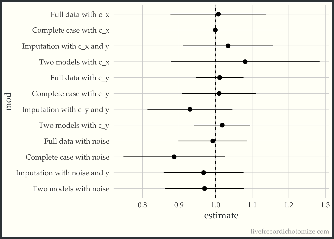
Pretty good! Maybe I’m feeling a little better about imputation. Maybe. But it had better include the outcome (which I’ll admit feels very weird for my little causal brain).